Handling Variable Time Series Efficiently in ClickHouse®


ClickHouse offers incredible flexibility to solve almost any business problem in a multiple of ways. Schema design plays a major role in this. For our recent benchmarking using the Time Series Benchmark Suite (TSBS) we replicated TimescaleDB schema in order to have fair comparisons. In that design every metric is stored in a separate column. This is the best for ClickHouse from a performance perspective, as it perfectly utilizes column store and type specialization.
Sometimes, however, schema is not known in advance, or time series data from multiple device types needs to be stored in the same table. Having a separate column per metric may be not very convenient, hence a different approach is required. In this article we discuss multiple ways to design schema for time series, and do some benchmarking to validate each approach. Our results show that these use cases can be optimized very nicely, though you should pay attention to trade-offs in each design.
Traditional schema
The schema we used for the original TSBS benchmark (see https://altinity.com/blog/clickhouse-for-time-series) is a straightforward one: every metric is stored in a separate column.
CREATE TABLE cpu (
  created_date Date DEFAULT today(),
  created_at DateTime DEFAULT now(),
  time String,
  tags_id UInt32,
  usage_user Float64,
  usage_system Float64,
  usage_idle Float64,
  usage_nice Float64,
  usage_iowait Float64,
  usage_irq Float64,
  usage_softirq Float64,
  usage_steal Float64,
  usage_guest Float64,
  usage_guest_nice Float64
) ENGINE = MergeTree(created_date, (tags_id, created_at), 8192);
We will start from there and see how other schema options compare.
Key-value arrays
One of the important ClickHouse features is array data types. For our purpose arrays can be used in order to store metrics as key-value pairs. Our main benchmarking table evolved as follows.
CREATE TABLE cpu_a (
  created_date Date,
  created_at DateTime,
  time String,
  tags_id UInt32,
  metrics.name Array(String),
  metrics.value Array(Float64)
) ENGINE = MergeTree(created_date, (tags_id, created_at), 8192);
Alternatively, we could define metrics using the Nested data type:
metrics Nested (
  name String,
  value Float64
)
Internally, it maps to two arrays exactly like the previous example.
So now instead of 10 columns we created two arrays. To make it simple we just move data to the new table with ‘INSERT … SELECT’. Note that this means we cannot measure ingestion performance with different schema designs, as it would require changes on the TSBS side. Ingestion is very fast in ClickHouse anyway, and it may be even better with a smaller number of columns, since every column is stored and compressed individually. We may come back to this question in a later article. Meanwhile, here is the SQL to move the data.
insert into cpu_a
select created_date, created_at, time, tags_id,
       array('usage_user', 'usage_system', 'usage_idle', 'usage_nice', 'usage_iowait', 'usage_irq', 'usage_softirq', 'usage_steal', 'usage_guest', 'usage_guest_nice'),
       array(usage_user, usage_system, usage_idle, usage_nice, usage_iowait, usage_irq, usage_softirq, usage_steal, usage_guest, usage_guest_nice)
from cpu;
A typical row now looks like:
Row 1:
───────€
created_date:  2016-01-01
created_at:    2016-01-01 00:00:00
time:          2016-01-01 00:00:00 +0000
tags_id:       6001
metrics.name:  ['usage_user','usage_system','usage_idle','usage_nice','usage_iowait','usage_irq','usage_softirq','usage_steal','usage_guest','usage_guest_nice']
metrics.value: [3,95,58,82,90,82,26,99,59,13]
In order to extract particular metrics we have to use array functions. For example, instead of:
max(usage_user)
we have to write
max(metrics.value[indexOf(metrics.name,'usage_user')])
Certainly, such an approach produces additional overhead. But to what extent? It turned out that uncompressed data size is twice as big, but compressed storage overhead is only 15% greater! In order to understand storage and compression numbers we run the following query:
SELECT
    table,
    sum(rows),
    sum(data_compressed_bytes) AS compr,
    sum(data_uncompressed_bytes) AS uncompr,
    uncompr / compr AS ratio
FROM system.parts
WHERE active AND (database = 'benchmark')
GROUP BY table
ORDER BY table;

┌─table─┬───€sum(rows)─┬───────€compr─┬──────€uncompr─┬───────────────€ratio─┐
│ cpu   │  103680000 │ 1292449419 │ 12130560000 │  9.385713530967976 │
│ cpu_a │  103680000 │ 1484871273 │ 25712640000 │ 17.316410161300226 │
└──────┴────────────┴────────────┴─────────────┴─────────────────────┘
(Note: we also run ‘OPTIMIZE TABLE FINAL’ for all tables to make sure the data is fully merged). Memory overhead is more significant, though, especially when the array size is large but only some metrics are extracted.
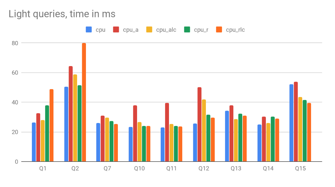
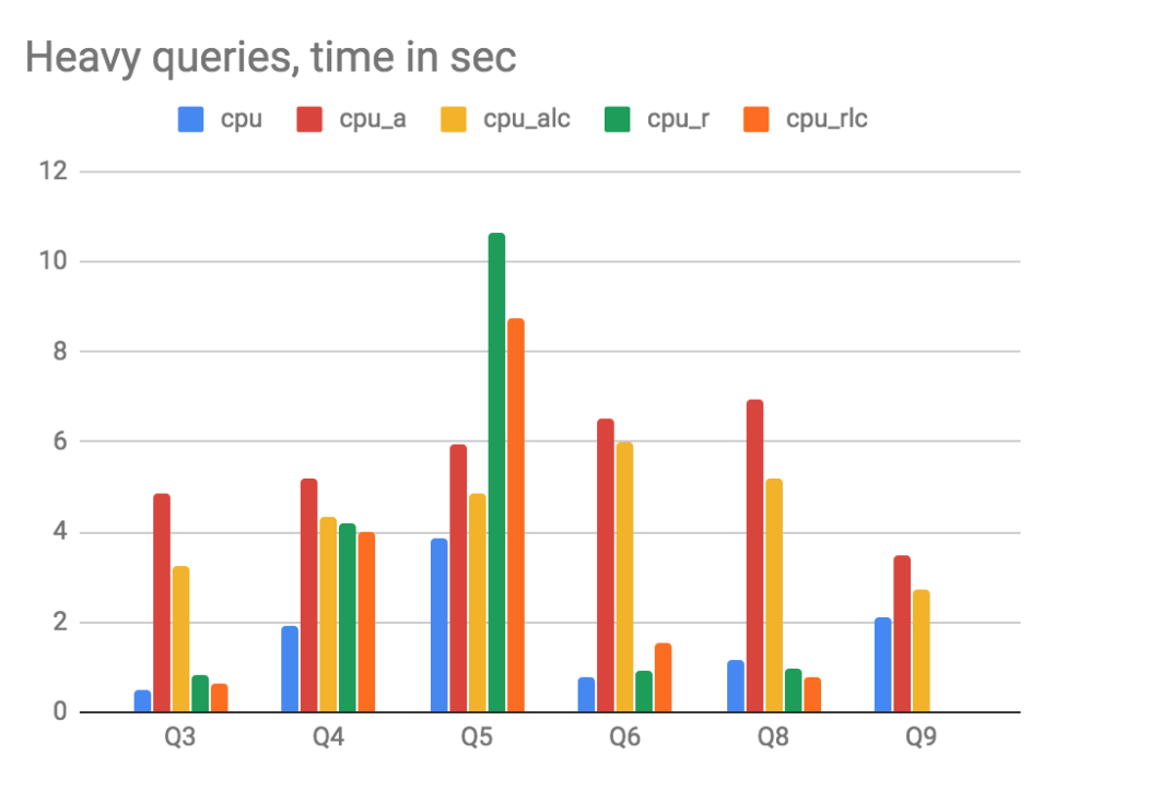
On the query side, we run a standard set of TSBS test queries. It turns out that performance is virtually unchanged for ‘light’ queries with millisecond time. Those queries mainly benefit from the index, and the storage model for metrics does not matter much. It is very different for ‘heavy’ queries though. All ‘heavy’ query include aggregation function applied to one or several metrics for a big portion of the dataset. This is where ClickHouse can be very fast aggregating scalar columns, but not that good with arrays. The performance for ‘heavy’ queries degrades significantly in our tests. Detailed results are available at the end of the article.
Fortunately, we can take advantage of ClickHouse flexibility to improve the schema design and raise performance.
Key-value arrays optimization
The approach with key-value arrays can be optimized for better response time. In particular, instead of strings for metric names it is possible to use some sort of integer based metric_ids. That will give better performance and also enable us to use the unique ClickHouse function sumMap() that takes two integer arrays, keys and values, and summarizes values by keys in an efficient way. A separate table for metrics definitions is required in this case, which adds complexity.
A better possibility is to use LowCardinality data type for metric names. LowCardinality is a new feature introduced in ClickHouse in Q4/2018. (For more information see the article that explains it in our blog: https://altinity.com/blog/2019/3/27/low-cardinality.) It is sometimes named dictionary encoding, because it stores integer keys in the table itself, while the dictionary is stored separately. In addition to space savings it enables optimizations in query time. Let’s see how it works.
CREATE TABLE cpu_alc (
  created_date Date,
  created_at DateTime,
  time String,
  tags_id UInt32,
  metrics Nested(
    name LowCardinality(String),
    value Float64
  )
) ENGINE = MergeTree(created_date, (tags_id, created_at), 8192);
Table sizes now look like this:
┌─table───┬───€sum(rows)─┬───────€compr─┬──────€uncompr─┬───────────────€ratio─┐
│ cpu     │  103680000 │ 1292449419 │ 12130560000 │  9.385713530967976 │
│ cpu_a   │  103680000 │ 1484871273 │ 25712640000 │ 17.316410161300226 │
│ cpu_alc │  103680000 │ 1482985574 │ 13893322653 │   9.36848132347375 │
└────────┴────────────┴────────────┴─────────────┴─────────────────────┘
It turns out that uncompressed size is almost two times better than array with string metric names and only 10% worse compared to the original flat table. Compressed is about the same as key-value array. So the effect is notable.
Performance of all test queries is slightly better than the plain array approach, in the 20% range. The difference should be not significant when array size grows. LowCardinality can not change the nature of arrays. It just makes it faster to search for proper metrics.
Metric per row
Another approach is to store every metric in a separate row. The table would look like the following.
CREATE TABLE cpu_r (
  created_date Date,
  created_at DateTime,
  time String,
  tags_id UInt32,
  metric_name String,
  metric_value Float64
) ENGINE = MergeTree(created_date, (metric_name, tags_id, created_at), 8192);
Note that ‘metric_name’ is now a part of the primary key. Otherwise it would be very slow to run an analysis for a single metric.
We can populate the data using the following query.
INSERT INTO cpu_r
SELECT created_date, created_at, time, tags_id, metric_name, metric_value
  FROM cpu_a
  ARRAY JOIN metrics.name AS metric_name, metrics.value AS metric_value;
The storage overhead is more pronounced now. Instead of 100M rows table we ended up with 1B rows in the table. Even though we have a better compression ratio, it does not help: the compressed size is almost 5 times larger than the reference flat table.
┌─table───┬───€sum(rows)─┬───────€compr─┬──────€uncompr─┬───────────────€ratio─┐
│ cpu     │  103680000 │ 1292449419 │ 12130560000 │  9.385713530967976 │
│ cpu_a   │  103680000 │ 1484871273 │ 25712640000 │ 17.316410161300226 │
│ cpu_alc │  103680000 │ 1482985574 │ 13893322653 │   9.36848132347375 │
│ cpu_r   │ 1036800000 │ 4705931212 │ 58475520000 │  12.42591898727482 │
└────────┴────────────┴────────────┴─────────────┴─────────────────────┘
Such a table is easy to query for a single metric, but if multiple metrics need to be retrieved, then we need to use yet another cool ClickHouse feature: the -If combinator. For example:
SELECT
    avgIf(metric_value, metric_name = 'usage_user') AS usage_user,
    avgIf(metric_value, metric_name = 'usage_system') AS usage_system
FROM cpu_r
WHERE metric_name IN ('usage_user', 'usage_system');
Note, we have to use ‘metric_name’ filter here as well, otherwise ClickHouse will scan all 1B rows. Using a filter reduces this amount to 200M for two metrics.
Performance-wise it showed mixed results again. From one side, it was able to outperform some of reference flat table tests when a single metric has been retrieved. Thanks to index and flat column for metric value. When multiple metrics need to be retrieved, however, the performance starts to degrade — ClickHouse has to process an extra 100M rows for every metric. For our test it is not that bad, but if the number of metrics is significantly higher it can be a serious issue. Another problem is querying related metrics, e.g. querying all metrics when one is above a certain threshold.
Metric per row with LowCardinality
Similar to the arrays approach, let’s now try LowCardinality datatype for metric_name.
CREATE TABLE cpu_rlc (
  created_date Date,
  created_at DateTime,
  time String,
  tags_id UInt32,
  metric_name LowCardinality(String),
  metric_value Float64
) ENGINE = MergeTree(created_date, (metric_name, tags_id, created_at), 8192);

┌─table───┬───€sum(rows)─┬───────€compr─┬──────€uncompr─┬───────────────€ratio─┐
│ cpu     │  103680000 │ 1292449419 │ 12130560000 │  9.385713530967976 │
│ cpu_a   │  103680000 │ 1484871273 │ 25712640000 │ 17.316410161300226 │
│ cpu_alc │  103680000 │ 1482985574 │ 13893322653 │   9.36848132347375 │
│ cpu_r   │ 1036800000 │ 4706173650 │ 58475520000 │ 12.425278867472304 │
│ cpu_rlc │ 1036800000 │ 4701044623 │ 46658930733 │  9.925226087988998 │
└────────┴────────────┴────────────┴─────────────┴─────────────────────┘
Storage is slightly better compared to simple String type. We see a 20% size reduction uncompressed and an insignificant performance increase–if any–since metric name is used in a filter already.
Mixed approach
Arrays are good but we have an unavoidable performance overhead. It is possible to have a hybrid approach and extract frequently used metrics as separate columns. For example, we can do the following:
CREATE TABLE cpu_alcm (
  created_date Date,
  created_at DateTime,
  time String,
  tags_id UInt32,
  metrics Nested(
    name LowCardinality(String),
    value Float64
  )
) ENGINE = MergeTree(created_date, (tags_id, created_at), 8192);
ALTER TABLE cpu_alcm add column
usage_user Float64 MATERIALIZED metrics.value[indexOf(metrics.name,'usage_user')];
Note the MATERIALIZED column keyword. Those columns can not be inserted. Instead they are calculated automatically during insertion or merge. So we can keep inserting data in the most general format using arrays, but have some columns extracted from the array automatically. There is a small overhead on storage due to the extra column:
┌─table────┬───€sum(rows)─┬───────€compr─┬──────€uncompr─┬───────────────€ratio─┐
│ cpu      │  103680000 │ 1292449419 │ 12130560000 │  9.385713530967976 │
│ cpu_a    │  103680000 │ 1484871273 │ 25712640000 │ 17.316410161300226 │
│ cpu_alc  │  103680000 │ 1482985574 │ 13893322653 │   9.36848132347375 │
│ cpu_alcm │  103680000 │ 1574346256 │ 14722762653 │    9.3516674599949 │
│ cpu_r    │ 1036800000 │ 4706173650 │ 58475520000 │ 12.425278867472304 │
│ cpu_rlc  │ 1036800000 │ 4701044623 │ 46658930733 │  9.925226087988998 │
│ tags     │      10000 │     102655 │      808080 │   7.87180361404705 │
└─────────┴────────────┴────────────┴─────────────┴─────────────────────┘
Query performance is certainly better when only the materialized metric is used. Once other metrics are involved the performance is back to the general array case.
Benchmarks
In order to measure performance of different schemes, we used queries from the Time Series Benchmark Suite. See our article that describes the approach in more detail: https://altinity.com/blog/clickhouse-for-time-series
Benchmarks were run at Intel(R) Core(TM) i7-7700 CPU 64Gb server with RAID10 disk array. To rule out I/O variation, all data was in the OS page cache during the test.
Test queries are summarized in the table below:
| # | Query tag | Description |
|---|---|---|
| Q11 | single-groupby-1-1-1 | Simple aggregate (MAX) on one metric for 1 host, every 5 mins for 1 hour |
| Q10 | single-groupby-1-1-12 | Simple aggregate (MAX) on one metric for 1 host, every 5 mins for 12 hours |
| Q12 | single-groupby-1-8-1 | Simple aggregate (MAX) on one metric for 8 hosts, every 5 mins for 1 hour |
| Q14 | single-groupby-5-1-1 | Simple aggregate (MAX) on 5 metrics for 1 host, every 5 mins for 1 hour |
| Q13 | single-groupby-5-1-12 | Simple aggregate (MAX) on 5 metrics for 1 host, every 5 mins for 12 hours |
| Q15 | single-groupby-5-8-1 | Simple aggregate (MAX) on 5 metrics for 8 hosts, every 5 mins for 1 hour |
| Q1 | cpu-max-all-1 | Aggregate across all CPU metrics per hour over 1 hour for a single host |
| Q2 | cpu-max-all-8 | Aggregate across all CPU metrics per hour over 1 hour for eight hosts |
| Q3 | double-groupby-1 | Aggregate on across both time and host, giving the average of 1 CPU metric per host per hour for 24 hours |
| Q4 | double-groupby-5 | Aggregate on across both time and host, giving the average of 5 CPU metrics per host per hour for 24 hours |
| Q5 | double-groupby-all | Aggregate on across both time and host, giving the average of all (10) CPU metrics per host per hour for 24 hours |
| Q8 | high-cpu-all | All the readings where one metric is above a threshold across all hosts |
| Q7 | high-cpu-1 | All the readings where one metric is above a threshold for a particular host |
| Q9 | lastpoint | The last reading for each host |
| Q6 | groupby-orderby-limit | The last 5 aggregate readings (across time) before a randomly chosen endpoint |
The test dataset contains 100M measurements for 10000 tags, and every measurement consists of 10 metrics. So table size varies from 100M to 1B rows depending on the schema approach:
- cpu — plain schema, every metric in a separate column
- cpu_a — schema with metrics.name/value arrays
- cpu_alc — similar to above, but metrics.name is LowCardinality(String)
- cpu_r — schema with every metric in a separate row.
- cpu_rlc — similar to above, but metric_name is LowCardinality(String)
Results are split into two graphs with different scale:
- Light queries typically execute below 100ms per query
- Heavy queries take several seconds per query
Conclusion
ClickHouse is very flexible and allows use of different designs for time series data. It is heavily optimized for well structured and properly typed schema, which is where the best query performance can be achieved. It allows, however, the use of semi-structured data as well, and the key-value array approach is a good design choice.
Using two distinct arrays — for metric names and metric values — shows just a small size overhead when LowCardinality(String) is used for names, and good performance. For simple lookups query performance degradation is hardly notable, but it is quite pronounced when heavy computational queries are used. Unlike plain columns, ClickHouse can not properly utilize its vectorized execution engine when processing arrays. Adding materialized columns, which can be added ‘on-the-fly’, can improve performance where necessary.
Schema layout is just a first but very important step of application design. Proper attention should be also paid to:
- Data types — see this Percona benchmark that highlights the importance of dat?types: https://www.percona.com/blog/2019/02/15/clickhouse-performance-uint32-vs-uint64-vs-float32-vs-float64/
- Materialized views for speeding up ‘last point’ or ‘asof’ queries — see https://altinity.com/blog/clickhouse-continues-to-crush-time-series
- Scaling out if one server is not enough — see https://altinity.com/blog/clickhouse-timeseries-scalability-benchmarks
ClickHouse is evolving rapidly. Exotic ASOF joins and time series-specific column encodings are already there. Stay tuned to learn about them soon!
ClickHouse® is a registered trademark of ClickHouse, Inc.; Altinity is not affiliated with or associated with ClickHouse, Inc.